Project 4 Ok Cupid
Code: GitHub
4.1 Introduction
This project analyzes data from on-line dating application OKCupid. In recent years, there has been a massive rise in the usage of dating apps to find love. Many of these apps use sophisticated data science techniques to recommend possible matches to users and to optimize the user experience. These apps give us access to a wealth of information that we’ve never had before about how different people experience romance.
The dataset okcupid_profiles.csv was provided by Kaggle.com: OkCupid Profiles
4.1.1 Project Goals
In this project, the goal is to analyze the data from Kaggle using tools of Data Science. The primary research question that will be answered is whether an OkCupid’s user astrological sign can be predicted using other variables from their profiles.
4.1.2 Analysis
This solution uses descriptive statistics and data visualization to find key figures in understanding the distribution, count, and relationship between variables. Since the goal of the project is to make predictions on the user’s astrological signs, classification algorithms from the supervised learning family of machine learning models are implemented.
4.2 Data
The project has one data set provided by Kaggle called okcupid_profiles.csv. In the data, each row represents an OkCupid user and the columns are the responses to their user profiles which include multi-choice and short answer questions.
To analyze the user profiles from OkCupid, pandas will be used to load the dataset into a DataFrame so that it can be explored and visualized with Python.
4.2.1 Data Characteristics
profiles has 59,946 rows and 31 columns, this is a good sign since there seems to be enough data for machine learning.
The columns in the dataset include:
TABLE 4.1: Description of variables in the dataset.
| Variable | Description |
| age | categorical variable of educational attainment |
| body_type | categorical variable of body type of user |
| diet | categorical variable of dietary information |
| drinks | categorical variable of alcohol consumption |
| drugs | categorical variable of drug usage |
| education | categorical variable of educational attainment |
| ethnicity | categorical variable of ethnic backgrounds |
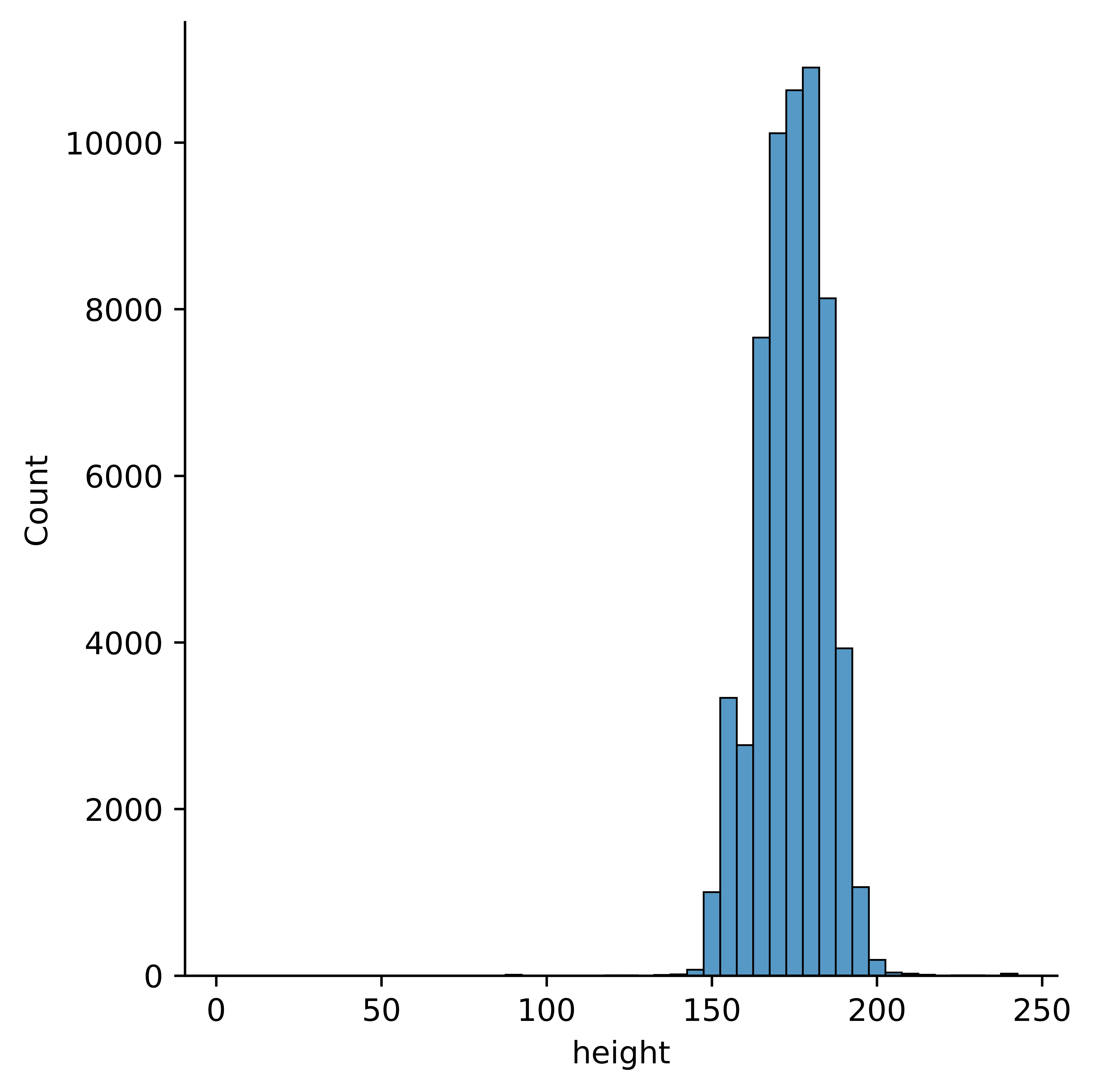
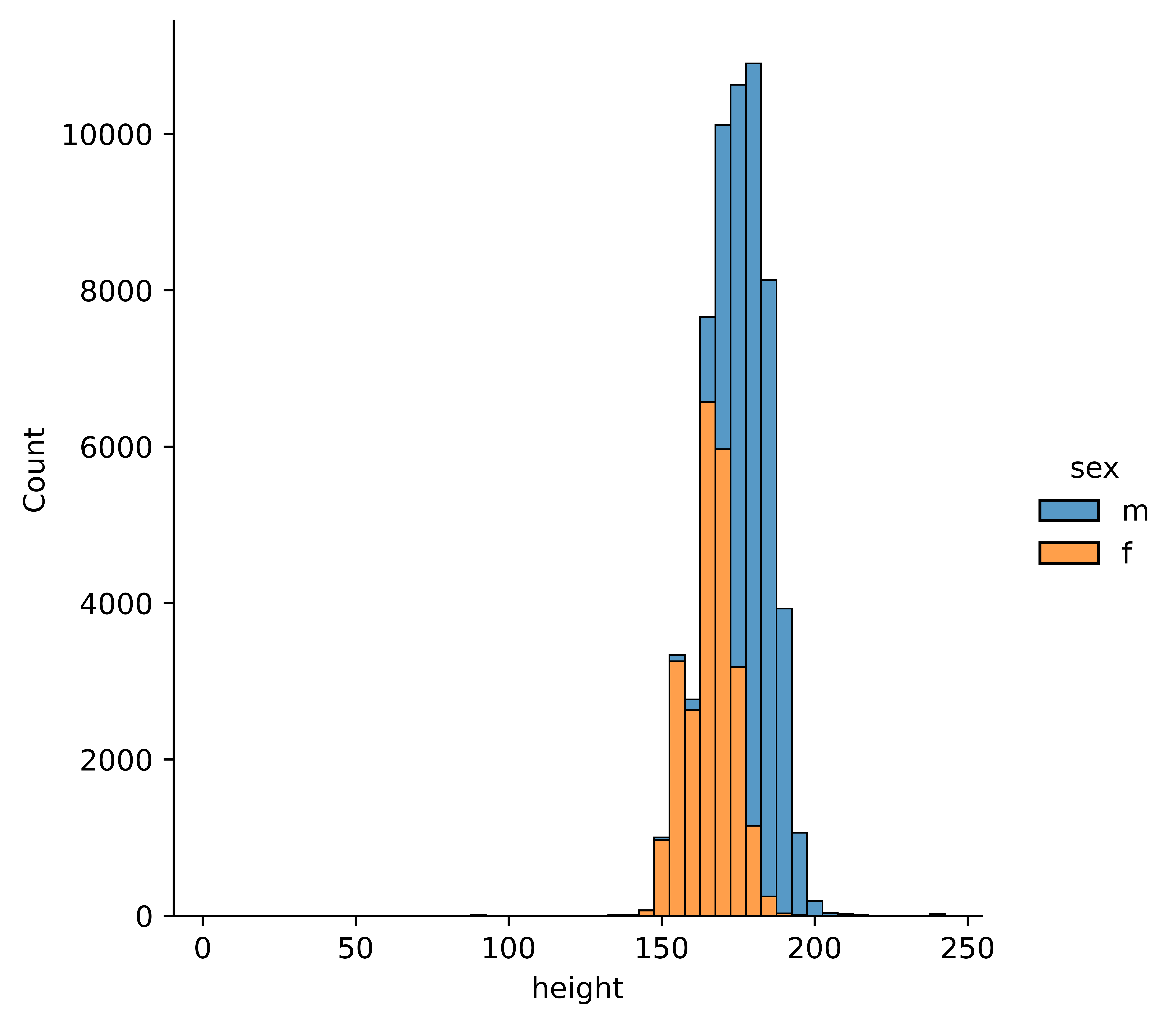
| height | continuous variable of height of user |
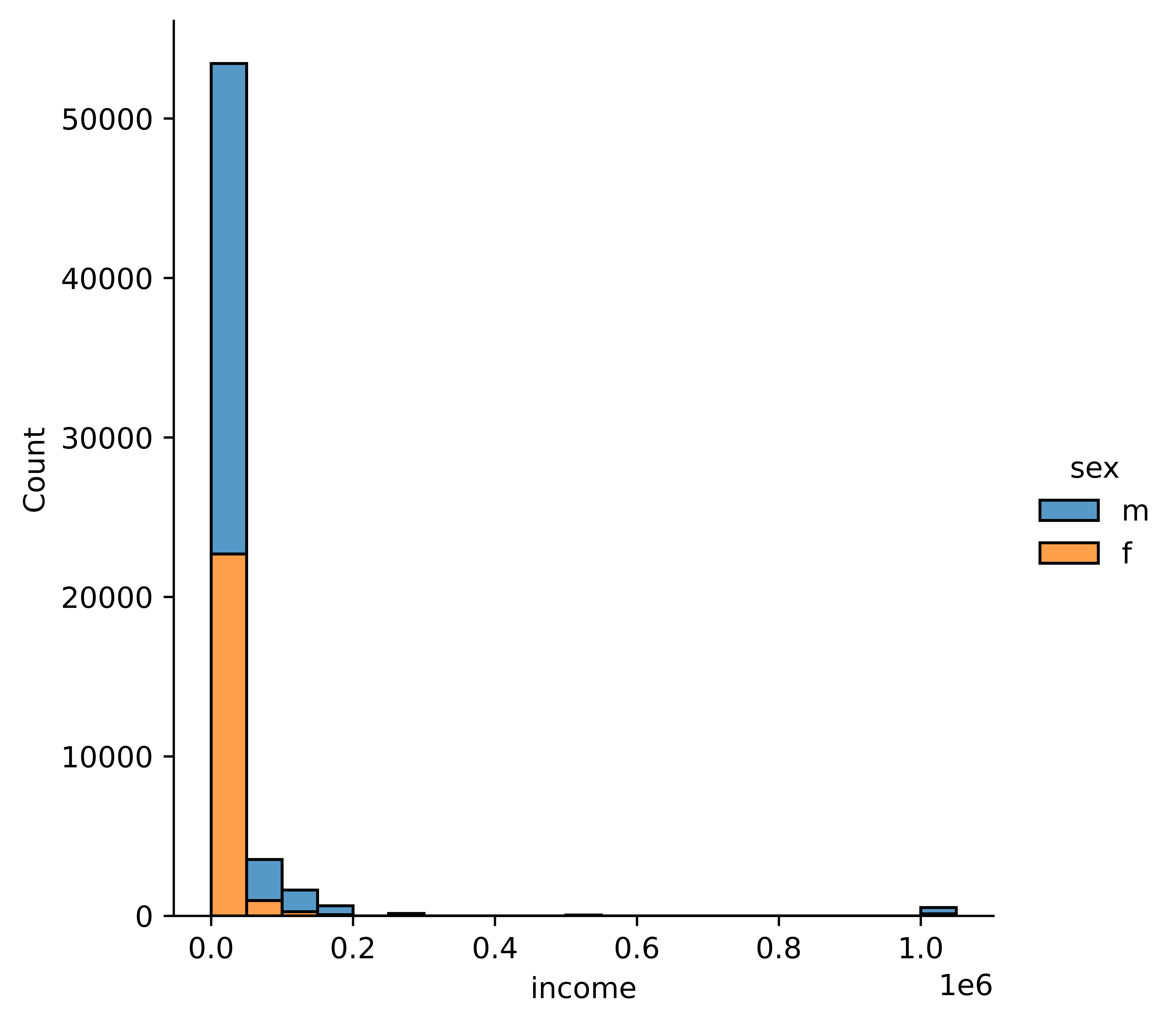
| income | continuous variable of income of user |
| job | categorical variable of employment description |
| offspring | categorical variable of children status |
| orientation | categorical variable of sexual orientation |
| pets: | categorical variable of pet preferences |
| religion | categorical variable of religious background |
| sex | categorical variable of gender |
| sign | categorical variable of astrological symbol |
| smokes | categorical variable of smoking consumption |
| speaks | categorical variable of language spoken |
| status | categorical variable of relationship status |
| last_online | date variable of last login |
| location | categorical variable of user locations |
And a set of open short-answer responses to :
TABLE 4.2: Description of variables short-answer in the dataset.
| Variable | Description |
|---|---|
| essay0 | My self summary |
| essay1 | What I’m doing with my life |
| essay2 | I’m really good at |
| essay3 | The first thing people usually notice about me |
| essay4 | Favorite books, movies, show, music, and food |
| essay5 | The six things I could never do without |
| essay6 | I spend a lot of time thinking about |
| essay7 | On a typical Friday night I am |
| essay8 | The most private thing I am willing to admit |
| essay9 | You should message me if… |
4.3 Exploring the Data
Let’s start by looking at the first rows and columns of our dataset:
TABLE 4.3: The 5 first lines of the Data Frame.
| age | status | sex | orientation | body_type | drinks | drugs | education |
|---|---|---|---|---|---|---|---|
| 22 | single | m | straight | a little extra | socially | never | working on college/university |
| 35 | single | m | straight | average | often | sometimes | working on space camp |
| 38 | available | m | straight | thin | socially | nan | graduated from masters program |
| 23 | single | m | straight | thin | socially | nan | working on college/university |
| 29 | single | m | straight | athletic | socially | never | graduated from college/university |
First to be explored is the number of unique signs, and the values. It seems that there are 48, but there should only be 12 signs.
It is important that we clean the labels since this is what will be predicted and 48 predictions would be quite difficult. By taking the first word of the column, the signs can be saved without the qualifiers. The qualifiers could be used for another problem down the line.
After adjusting the signs, we can better analyze them on our dataset.
4.3.1 Continuous Variables
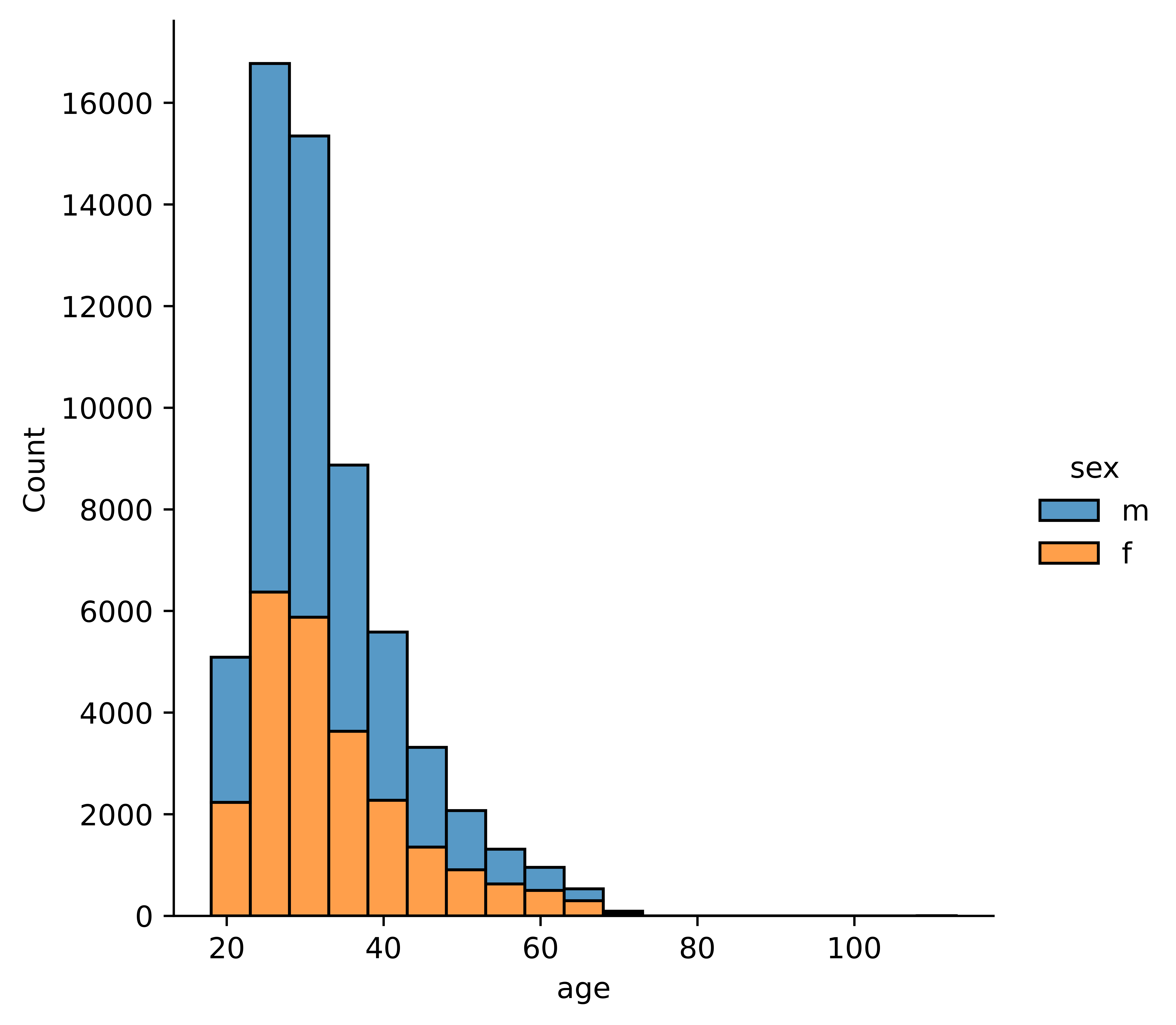
4.3.1.1 age
The next plot shows the distribution of age in the group. It seems that most users are in their late 20s to early 30s.

Here is the same chart but broken down by gender. It seems that there are proportionally similar breaks of gender by age, but slightly fewer females overall.
4.3.2 Discrete Variables
4.3.2.1 Sex
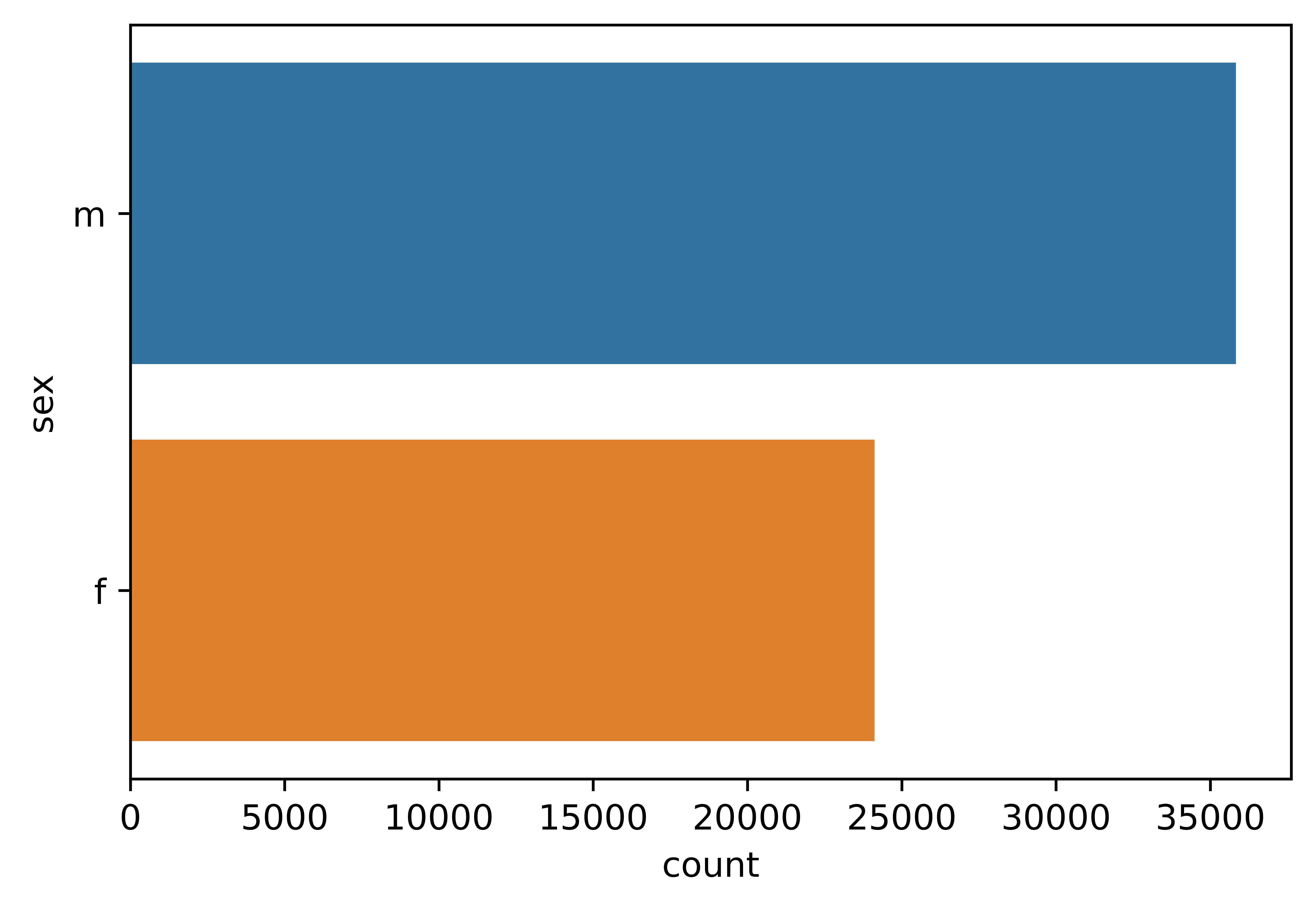
Previously it was identified that there are more males in the data, and it seems that there are ~35,000 men to ~25,000 women.
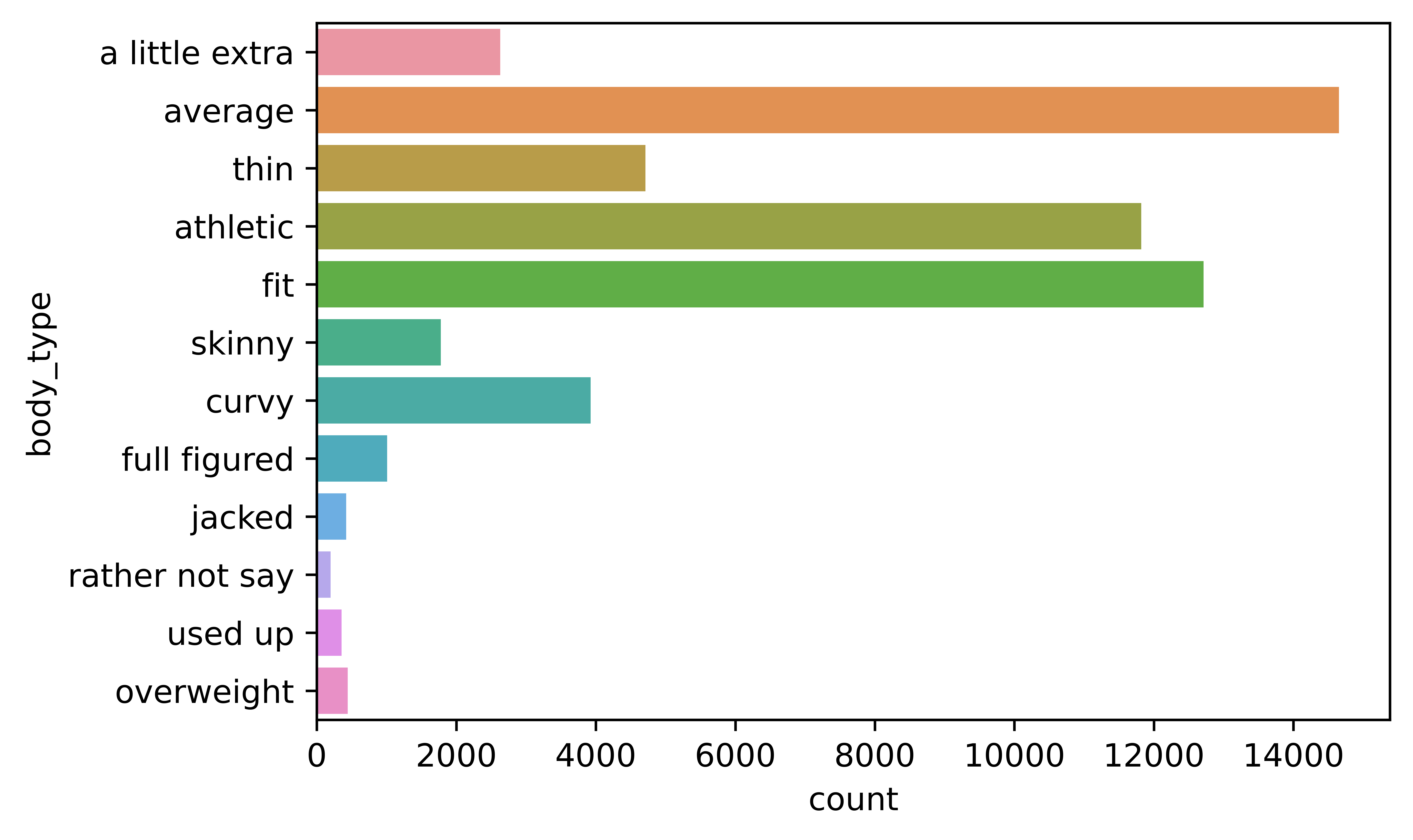
4.3.2.2 Body Type
The next chart shows the body type variable, and it seems that most users will describe themselves as average, fit, or athletic.
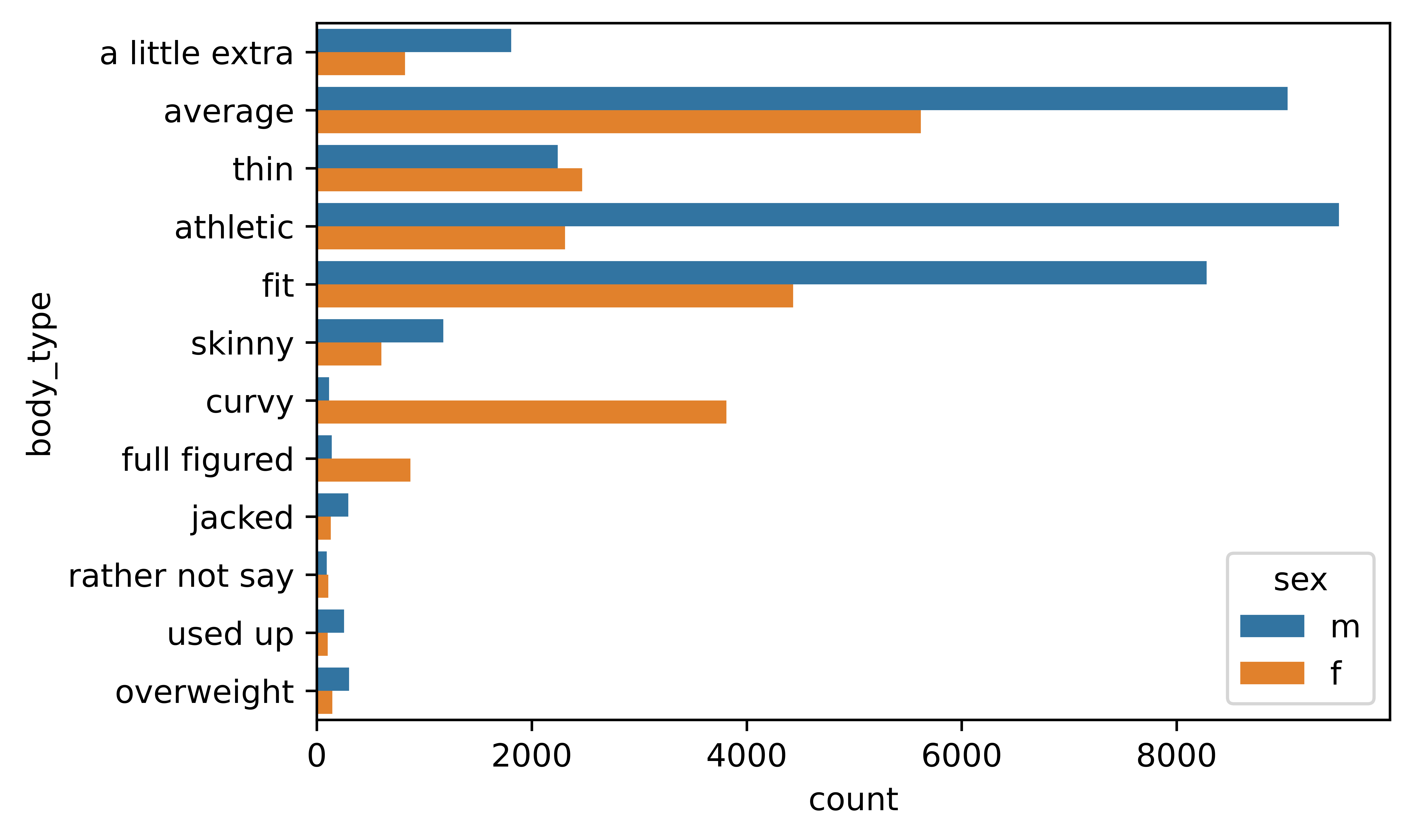
The next chart shows the breakdown of body type by gender and it seems that some of the body type descriptions are highly gendered. For example “curvy” and “full figured” are highly female descriptions, while males use “a little extra”, and “overweight” more often.
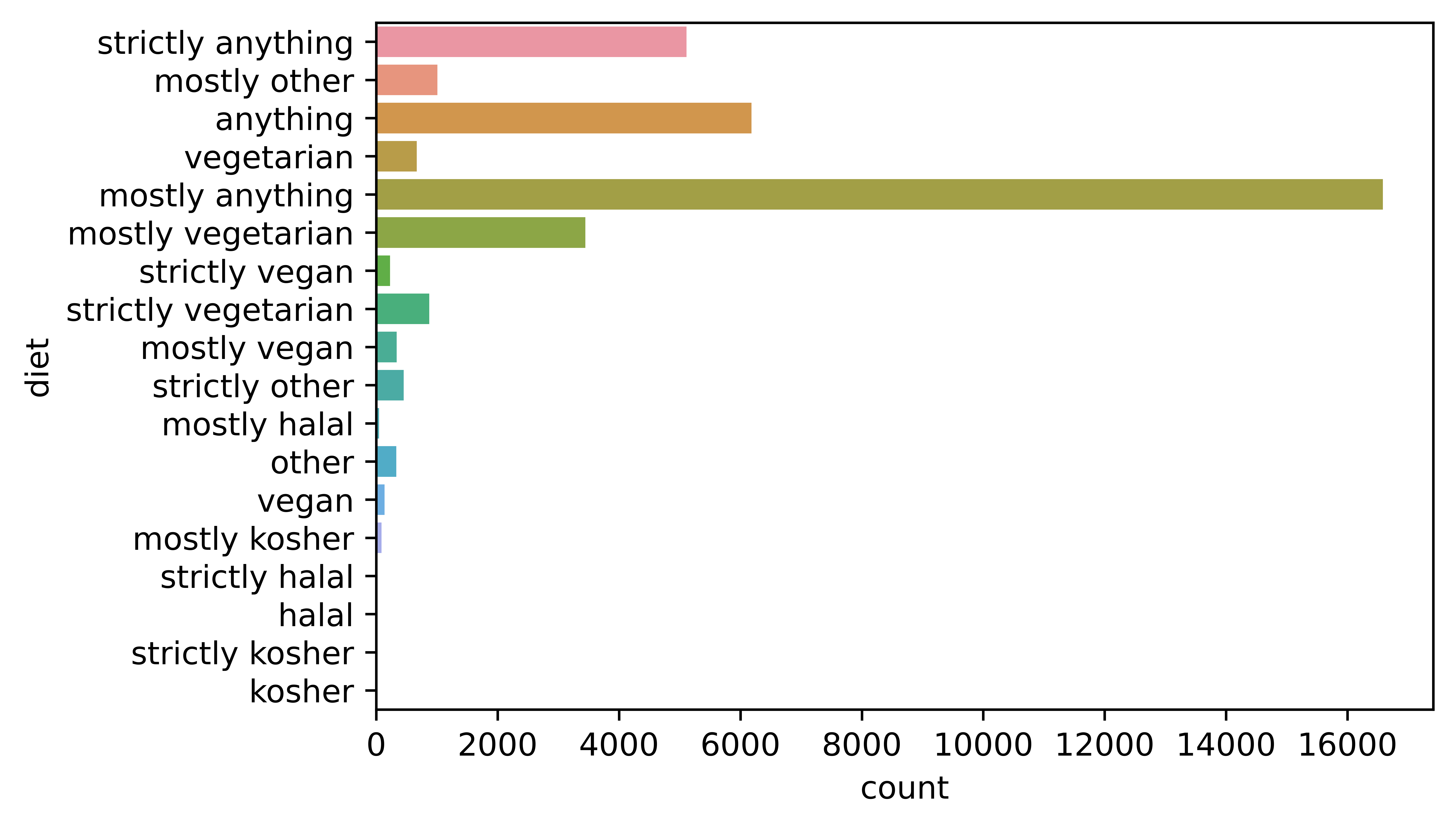
4.3.2.3 Diet
Here is a chart of the dietary information for users. Most users eat “mostly anything”, followed by “anything”, and “strictly anything”, being open-minded seems to be a popular signal to potential partners.
4.3.2.4 Drinks
The next plot shows that the majority of the users drink “socially”, then “rarely” and “often”.
4.3.2.7 Education
Below you can see the majority of users are graduates from college/university followed by masters programs and those working on college/university. Interestingly space camp related options are fairly popular options.
4.3.2.8 Jobs
Most users don’t fit into the categories provided, but there are a fair share of students, artists, tech, and business folks.
4.3.2.12 Religion
Religion was similar to sign where there are a lot of qualifiers.
religion was cleaned to take the first word and distilled down to 9 groups. The majority was not very religious identifying as agnostic, other, or atheists.
4.4 Data Preparation
Missing data is often not handled by machine learning algorithms well and have to be checked so they may need to be imputed or removed. It seems that many of the columns do have missing values.
Preparing the data for modeling is important since it can speed up the process and produce better models. As the adage goes, “garbage in garbage out” so we want to make sure the data we are inputting into our modelling step is good enough to share with others.
The data for the model is going to be a subset of the variables. The variables were selected because they might be a good predictor for astrological signs, where some of the variables that were not selected such as age is probably not a good indicator.
Missing values are dropped to create a fully complete data set.
Furthermore, an imbalance in the prediction label needs to be checked. This is important since it’s a multi-class problem where two or more outcomes can be bad. An imbalance in a response variable is bad since it means that some labels only occur a few times. This is an issue for machine learning algorithms if there is not enough data to train with which will give bad predictions.
In the given dataset, we observe that the counts of all the zodiac signs are more or less equal (i.e., without large deviations). Hence, we do not have to worry about imbalances and trying to address this problem.
Next the data was split into train and validation sets. In this split 25% of the data is reserved for the final validation, while 75% is kept for training the model.
4.5 Prediction
4.5.1 Model building
Now it’s time to create some models, here is a list of Multi class models available in scikit learn. For this project three common algorithms will be used to make predictions.
Below, the respective modules for Logistic Regression, Decision Trees, and KNN are loaded.
4.5.2 Evaluation Metrics
In the models, there will be several values that can be evaluated below is a quick diagram:  here is a quick description of the metrics:
- Accuracy: is the correct values divided by total values
- Precision: is the True Positives divided by the sum of True Positives and False Negatives. So precision is the values of the true positives divided by the actual positive values.
- Recall: is the True Positives divided by the sum of True Positives and False Positives. So recall is the values of the true positives divided by the positive guesses.
- F1-score: is a blended score of precision and recall which balances both values.
- Macro Avg: is the unweighted mean value of precision and recall.
- Weighted Avg: is the weighted mean value of precision and recall by the support values for each class.
- Support: is the number of observations in class to predict.
4.5.3 Logistic Regression
The first model is using logistic regression with the multi_class="multinomial" argument. Using lr_model predictions are created from the training dataset which is used to figure out how well the model performed.
              precision    recall  f1-score   support

    aquarius       0.13      0.06      0.08       930
       aries       0.13      0.11      0.12      1012
      cancer       0.13      0.20      0.15      1067
   capricorn       0.14      0.05      0.08       921
      gemini       0.12      0.12      0.12      1116
         leo       0.12      0.18      0.15      1123
       libra       0.13      0.12      0.13       992
      pisces       0.12      0.11      0.12      1026
 sagittarius       0.12      0.06      0.08       993
     scorpio       0.12      0.08      0.09      1013
      taurus       0.12      0.14      0.13      1051
       virgo       0.13      0.21      0.16      1095

    accuracy                           0.12     12339
   macro avg       0.12      0.12      0.12     12339
weighted avg       0.12      0.12      0.12     12339
The final accuracy of the logistic regression model is 12% which is terrible considering a random guess should result in being correct ~8% of the time (1/12).
4.5.4 K Nearest Neighbor
The next model is the KNeighborsClassifier which will take 20 of it’s neighbors to predict the signs. The default value for n_neighbors is 5 which was kept. This number can be tuned later on if needed.
              precision    recall  f1-score   support

    aquarius       0.26      0.66      0.37       930
       aries       0.26      0.53      0.35      1012
      cancer       0.30      0.44      0.35      1067
   capricorn       0.34      0.37      0.35       921
      gemini       0.34      0.32      0.33      1116
         leo       0.40      0.28      0.33      1123
       libra       0.38      0.23      0.29       992
      pisces       0.42      0.25      0.31      1026
 sagittarius       0.43      0.23      0.30       993
     scorpio       0.42      0.22      0.29      1013
      taurus       0.42      0.25      0.31      1051
       virgo       0.42      0.23      0.29      1095

    accuracy                           0.33     12339
   macro avg       0.36      0.33      0.32     12339
weighted avg       0.37      0.33      0.32     12339
This model had a 33% accuracy which is a good sign.
4.5.5 Decision Trees
The last model is the decision tree, the default max_depth is none which means that it will “If None, then nodes are expanded until all leaves are pure or until all leaves contain less than min_samples_split samples.”.
              precision    recall  f1-score   support

    aquarius       0.66      0.94      0.78       930
       aries       0.67      0.89      0.76      1012
      cancer       0.70      0.87      0.78      1067
   capricorn       0.73      0.84      0.78       921
      gemini       0.76      0.79      0.78      1116
         leo       0.80      0.79      0.80      1123
       libra       0.79      0.76      0.78       992
      pisces       0.81      0.74      0.77      1026
 sagittarius       0.88      0.70      0.78       993
     scorpio       0.89      0.71      0.79      1013
      taurus       0.94      0.67      0.78      1051
       virgo       0.91      0.67      0.77      1095

    accuracy                           0.78     12339
   macro avg       0.80      0.78      0.78     12339
weighted avg       0.80      0.78      0.78     12339
The results are very promising because it has a 78% accuracy with this model.
Below is a confusion matrix of the results with the true values on the y axis and predicted values along the x axis. Since the diagonals are lighter in color and have higher numbers, the accuracy is going to be high since those are the True Positives.
Going back to the model, a quick analysis shows that this tree model has a depth of 65 branches, which probably not generalize to another dataset. In this case this model has been “overfit” for this data.
To make a point, a five fold cross validation is created with the same data. The results are worse than the KNN and about the Logistic Regression algorithms. the baseline was ~9%
The decision tree model will be made again, but with a max_depth of 20 to stop the algorithm from reaching the stopping point.
              precision    recall  f1-score   support

    aquarius       0.40      0.33      0.36       930
       aries       0.40      0.27      0.32      1012
      cancer       0.40      0.28      0.33      1067
   capricorn       0.27      0.30      0.28       921
      gemini       0.37      0.26      0.31      1116
         leo       0.37      0.25      0.30      1123
       libra       0.59      0.19      0.29       992
      pisces       0.19      0.44      0.26      1026
 sagittarius       0.40      0.23      0.29       993
     scorpio       0.64      0.20      0.30      1013
      taurus       0.39      0.25      0.31      1051
       virgo       0.16      0.47      0.24      1095

    accuracy                           0.29     12339
   macro avg       0.38      0.29      0.30     12339
weighted avg       0.38      0.29      0.30     12339
The new accuracy rate of ~41% is worse than the first iteration, but slightly better than the KNN model.
If we check again with cross validation, the new model is still averaging ~8% which is not very good.
              precision    recall  f1-score   support

    aquarius       0.08      0.20      0.11       332
       aries       0.09      0.18      0.12       316
      cancer       0.09      0.13      0.11       390
   capricorn       0.05      0.06      0.05       276
      gemini       0.08      0.08      0.08       380
         leo       0.10      0.07      0.08       393
       libra       0.08      0.05      0.06       362
      pisces       0.07      0.04      0.05       308
 sagittarius       0.09      0.04      0.06       319
     scorpio       0.07      0.03      0.05       343
      taurus       0.08      0.05      0.06       339
       virgo       0.14      0.08      0.10       356

    accuracy                           0.08      4114
   macro avg       0.09      0.08      0.08      4114
weighted avg       0.09      0.08      0.08      411
4.5.6 Final Model
So it seems that the knn_model might be the best model for OkCupid to use when users don’t have their signs listed on their user profile. By using the hold out or validation set, we get ~8% accuracy which is not very good.
precision    recall  f1-score   support

    aquarius       0.08      0.22      0.12       294
       aries       0.09      0.18      0.12       345
      cancer       0.09      0.15      0.11       328
   capricorn       0.06      0.06      0.06       315
      gemini       0.08      0.06      0.07       366
         leo       0.10      0.07      0.08       395
       libra       0.10      0.06      0.08       326
      pisces       0.07      0.05      0.06       337
 sagittarius       0.08      0.03      0.05       347
     scorpio       0.08      0.04      0.05       355
      taurus       0.07      0.04      0.05       345
       virgo       0.08      0.05      0.06       361

    accuracy                           0.08      4114
   macro avg       0.08      0.08      0.08      4114
weighted avg       0.08      0.08      0.07      4114
In the confusion matrix, it becomes clear that Cancer, Gemini, Leo, and Virgo was predicted most often, but were not super accurate since the vertical color band represents even distributed guesses mostly wrong and some correct.
4.6 Conclusion
In this project, machine learning was used to predict the astrological signs of OkCupid users. This is an interesting feature, as many people believe in astrology and combinations between compatible star signs. If users do not enter their signals, an algorithmic solution may have generated a signal to input the missing data when making matches.
Unfortunately, the final algorithm selected was no better than basic guessing, showing that not everything is appropriate for using machine learning as many people say out there.